Is exponent 2.0 actually optimal? Where 1.83 came from, and a first taste of overfitting
Last post ended with this question.
Is 2.0 actually the right exponent? Can we find the real best from the data?
Bill James used RS² / (RS² + RA²), and we saw it fit our 5 seasons well. But why squared? James himself admitted it wasn't derived — he picked it because it worked. Some baseball analysts use 1.83 instead. Who's right?
This post in one sentence:
2.0 is a bit too high, 1.83 is reasonable, and on our 5-season data the best is 1.71. But the difference is around 0.1 wins per season — practically nothing. And that's the most important part of this post.
The exponent is a number we get to choose
A quick concept aside. The Pythagorean expectation generalizes to:
Bill James fixed k = 2, but that 2 didn't come from anywhere fundamental. We get to pick it. In data analysis, a number we set ourselves inside a model is called a hyperparameter. The shape of the formula is fixed, the dial inside it is for us to turn.
Once you start doing machine learning, hyperparameters are everywhere — learning rate, regularization strength, tree depth. The essence is the same. A degree of freedom no one else has set, so we have to look at the data and decide.
Which leads to the natural next question. Sweep k from 1.5 to 2.5 in 0.01 steps and find which value best fits actual win rates.
What do we mean by "best fits"
We already picked our answer last post. MAE — Mean Absolute Error.
The average absolute difference between each team's actual win rate and the Pythagorean prediction. Multiply by 162 and you get "how many wins off, on average, the prediction is."
Same reason as last post — r barely moves between 0.9503 and 0.9511, but MAE gives a direct answer to "did this drop from 3.5 wins off to 3.0 wins off?"
When you're comparing different models against each other, an error metric like MAE is cleaner than r.
A curve appears
We tested all 101 values of k from 1.50 to 2.50, computing MAE across all 5 seasons (150 teams) at each value. Plot k on the x-axis and MAE on the y-axis:
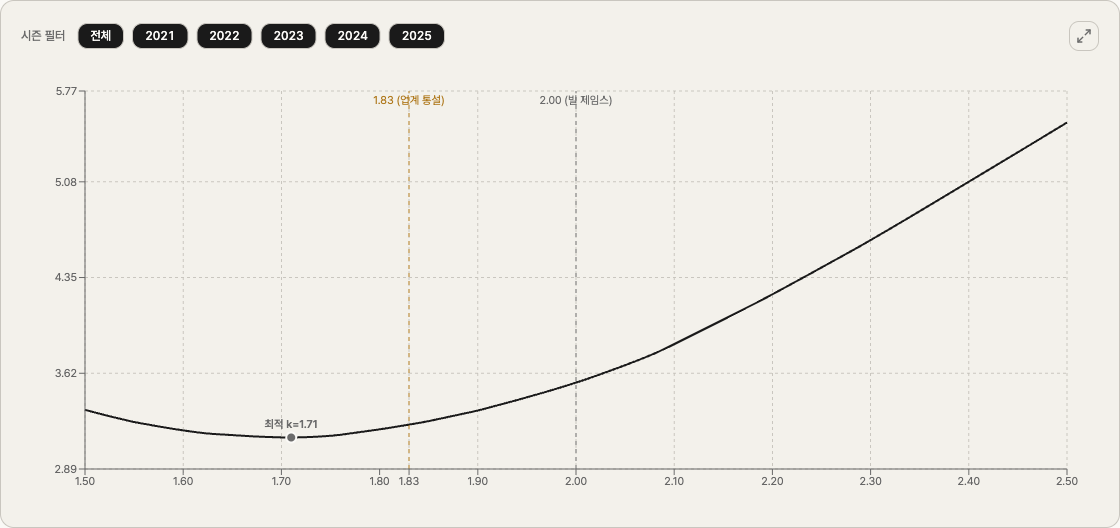
The shape is clean. It drops on the left, hits a floor somewhere in the middle, then climbs again. A U-curve.
The bottom of that U is the optimum our data points to. It sits at k = 1.71.
At that k, MAE is 0.01932 — about 3.13 wins per season. Bill James' 2.00 lands at 3.55 wins; the industry-standard 1.83 lands at 3.23. Side by side:
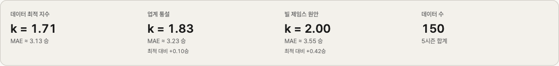
| Exponent | MAE (wins) | Vs. optimum |
|---|---|---|
| Data optimum 1.71 | 3.13 | — |
| Industry 1.83 | 3.23 | +0.10 wins |
| Bill James 2.00 | 3.55 | +0.42 wins |
Read literally: "1.71 is best, 2.00 misses by 0.42 wins more." But 0.42 wins is the gap in average per-team error per season. Across 162 games, that's almost noise.
The 1.83 vs 1.71 gap of 0.10 wins is even smaller. Practically interchangeable.
Where 1.83 came from, by the way
A small story. The origin of 1.83 is more interesting than you'd expect.
It came from Daryl Morey. Basketball fans know him as the longtime Houston Rockets GM, currently the Philadelphia 76ers' President of Basketball Operations. Before basketball, Morey did baseball analytics. In the late 1990s, looking at Bill James' k = 2, he asked the same question we asked: "why exactly 2?" So he ran the same kind of sweep on a much larger historical dataset (going back to the early 1900s) and found that MAE bottomed out near 1.83.
Major stat sites like Baseball Reference adopted Morey's 1.83 over James' 2 as the default. So 1.83 isn't a number someone pulled out of the air — it's the result of doing exactly the work this post is doing, on bigger data.
Which means our 1.71 from 5 seasons isn't really a "discovery" either. The optimum drifts as the data sample changes. Morey's 1.83 came from ~100 years of seasons; our 1.71 came from 5.
That naturally invites the next suspicion.
What about a single season — how much would the optimum shift if we only used 30 teams?
One season at a time — 1.57 through 1.76
If 1.71 is the answer when we pool 5 seasons, what happens if we re-run the sweep on each individual season (30 teams)?
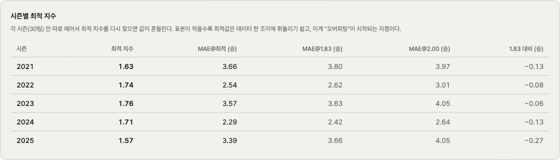
| Season | Optimum k |
|---|---|
| 2021 | 1.63 |
| 2022 | 1.74 |
| 2023 | 1.76 |
| 2024 | 1.71 |
| 2025 | 1.57 |
A range of 1.57 to 1.76. A spread of 0.19. The mean is around 1.68, and our pooled 1.71 sits right where it should — the natural average.
Why does it move season to season? Each season is 30 teams. Statistically, that's a small sample. The randomness inside it — who happened to win a lot of one-run games, who slumped in August and recovered in September — sways "the optimum for that season."
This is our first encounter with a fundamental concept in data analysis. Overfitting.
Overfitting — when a model "memorizes"
Overfitting in one sentence:
A model that has memorized the random noise in the data, not just the underlying pattern.
Each season's optimum k fits that season's MAE perfectly. Use k = 1.57 on the 2025 30-team set, and you get the lowest possible MAE for 2025. But take that 1.57 and apply it to 2024? It will probably do worse than 2024's own optimum (1.71). 1.57 has memorized 2025's randomness, and that randomness doesn't repeat next year.
This trap is everywhere in data analysis.
- A retail sales model with 12 variables that hits r² = 0.99 — it might just be memorizing last year's revenue
- A machine learning model with 99.9% training accuracy that drops to 60% on new data — memorized
- Our case here, where each season's optimum k differs — likely fitting season-specific noise
The simplest cure for overfitting is "tune less." If our per-season optima range from 1.57 to 1.76, instead of nailing down one value, picking a sensible value somewhere in that band is fine. 1.83 sits right there. It's a touch above our 5-season optimum, but Morey's longer-history work showed it's the stable plateau.
Stopping short of the perfect-fit value, and settling for a sensible one, often does better on future data. Counterintuitive, but a lesson that comes up again and again the deeper you go in data analysis.
Summing up
What we did this post in five lines.
- Swept k in the Pythagorean formula from 1.50 to 2.50
- Our 5-season data points to k = 1.71 as the optimum
- That's 0.42 wins better than James' 2.00 and 0.10 wins better than the industry's 1.83
- Per-season optima drift between 1.57 and 1.76 — the limit of small samples
- Which is why the industry's 1.83 — a not-quite-optimal but stable value — is actually the safer pick
Along the way we met two concepts that will follow us through the rest of this series. Hyperparameter and overfitting.
A bridge to next
Last post left a thread hanging.
A residual of +0.091 isn't all luck. Some of it is skill, some is luck. How do we tell them apart?
We can't answer it directly. But the next season gives us a hint. If a team got truly lucky in one season, it should regress next year. If what looked like luck was actually skill, it should show up the same way again.
The 2021 Mariners (+14.8 wins, residual +0.091) — what happened in 2022? The 2023 Padres (−11 wins) — did they recover in 2024?
Next post is on regression to the mean. The name sounds technical, but the phenomenon is something everyone intuitively knows. We'll watch the data confirm that intuition, and along the way figure out how we might begin to separate luck from skill.
This analysis is on the Q3 page of just-mlb, a tool I built. You can play with the MAE curve and the per-season table directly — toggling individual seasons via the season-filter chips is a fun way to see how the curve wobbles.